In the last post, I mapped gas stations and gas prices in Germany. After posting it, I started to look at the dataset from a different angle. The starting question was; “How can I model gas prices? What are the influencing factors?” One well known fact is that certain gas station brands demand higher prices.

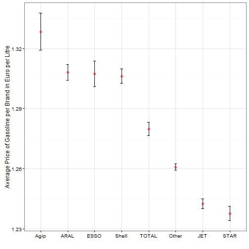
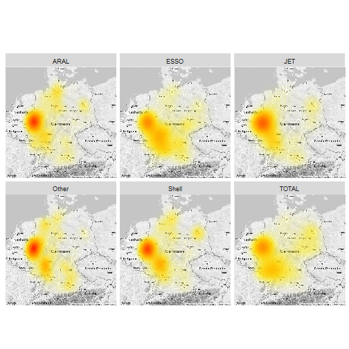
That is also the case in the present data. All but one of major brands have higher prices than the non-brand (“other”) gas stations. As an interesting fact, apparently, these brands have their home turfs, as illustrated by the following map.

From the data, we can also calculate the distance between each station. Peter Rosenmai provides a very nice function to do that for all station combinations (2792 * 2792). On my pretty old laptop it takes roughly 30 minutes to calculate the 8 million distances. From that we can count how many stations are within a certain distance from a single station. For example, there are on average ~8 other gas stations within a 5 kilometer radius. I created three variables, dist5 (5 kilometer radius, dist10, 10 km radius and dist20). In order to see which of these variables has predictive power on the gas price, we can run a simple “horse-race” regression on the price.

summary(lm(price ~ dist5 + dist10 + dist20, data=df4))

## 
## Call:
## lm(formula = price ~ dist5 + dist10 + dist20, data = df4)
## 
## Residuals:
##       Min        1Q    Median        3Q       Max 
## -0.112957 -0.042385 -0.019434  0.006249  0.286630 
## 
## Coefficients:
##                Estimate  Std. Error t value             Pr(>|t|)    
## (Intercept)  1.31952601  0.00226420 582.778 < 0.0000000000000002 ***
## dist5       -0.00019993  0.00040290  -0.496               0.6198    
## dist10      -0.00061953  0.00026656  -2.324               0.0202 *  
## dist20      -0.00048398  0.00007588  -6.378       0.000000000209 ***
## ---
## Signif. codes:  0 '***' 0.001 '**' 0.01 '*' 0.05 '.' 0.1 ' ' 1
## 
## Residual standard error: 0.07342 on 2788 degrees of freedom
## Multiple R-squared:  0.1283,	Adjusted R-squared:  0.1274 
## F-statistic: 136.8 on 3 and 2788 DF,  p-value: < 0.00000000000000022

We see that both the 10km and 20km variables carry weight and significance. That result is also clearly visible by plotting the gas price by the number of competitors within 20km.

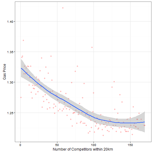
The posted gas price decreases from 1.33 to 1.25 for no competition to 100 competitors in close proximity. One way to cross-validate the result, is to split the gas stations in 4 similar sized groups and check if the result holds. I do that by splitting the stations by their median(latitude/longitude). The map illustrates that.

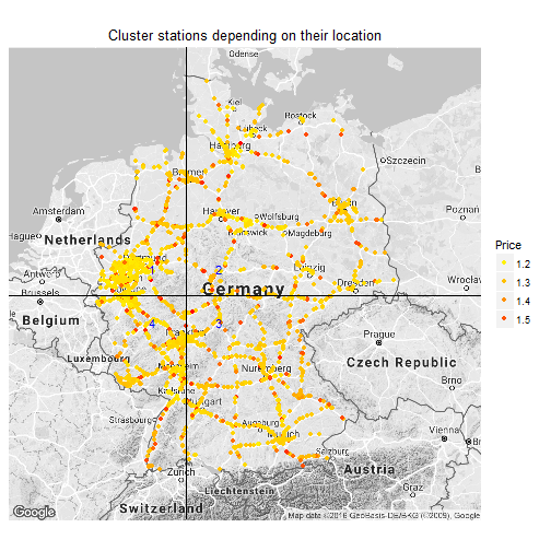
I use the blue numbers to label/group the stations according to their location. Then I do the same plot; gas price by the number of competitors within 20km for each quadrant separately.

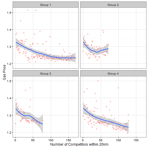
Overall the results hold. Prices decrease with increasing local competition. One factor biasing the analysis is that inner-city gas stations are known to have lower prices compared to stations along the “Autobahn”. I somewhat controlled for that by just including gas stations which are positioned at the Autobahn. It might be interesting to re-run the analysis on a wider dataset.

To come back to the starting question; What are the key gas price influencing factors? We can do a simple model comparison using the awesome BayesFactor package. The plot shows all models and ranks them according to their BayesFactor (higher is better).

reg <- generalTestBF(price ~ dist5 + dist10 + dist20 + brand, data=df4)
plot(reg /reg[4], logbase = "ln")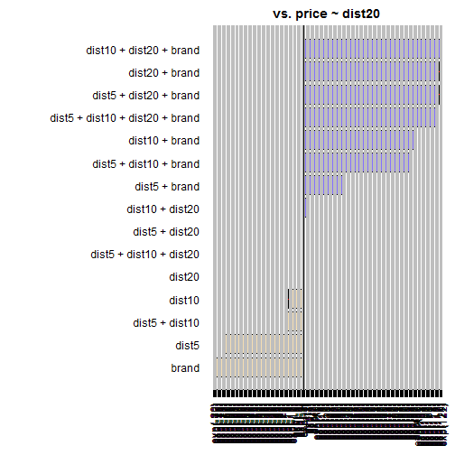

We see that the single most important factor is the number of close competitors in 20km (dist20). Also, the best model includes dist10 and brand, but excludes dist5.

Hence, the next time you see low gas prices, you know it is because the high regional competition ;).