Associated Keywords: The Missed Opportunity in Search Advertising
Short practical advise on search advertising:
-
Look beyond brand and category keywords The paper shows “associated keywords” — terms like “license,” “battery,” “plates” — are searched 50-80 days before purchase, have high category purchase probability, and cost significantly less than brand or category terms.
-
Just a few days of search history dramatically improves targeting Models using 5 days of search history achieve 8-15 percentage point improvement in predicting conversion compared to single-query targeting. The returns diminish quickly after 7 days.
-
Ad effectiveness varies by journey stage and keyword type Brand keywords work best at purchase (1.5x lift), but associated keywords provide meaningful lift earlier in the journey when the gap between category and brand commitment is highest.
-
Target the “commitment gap” The biggest opportunity is people committed to buying in the category but not yet committed to a specific brand. This gap is widest early in the journey, which is precisely where advertisers currently spend the least.
Long Version
A recent paper by Rothschild, Needell, Veverka, and Yom-Tov (2025) maps conversion journeys using a massive corpus of Bing search queries. What I found interesting is how clearly it shows that advertisers are concentrating their spend on people who are already likely to buy, while ignoring earlier stages of the journey where the marginal return on advertising could be much higher.
The authors introduce “associated keywords” — terms related to the conversion journey but not the actual products, brands, or product categories. These terms represent a largely untapped opportunity for targeting people committed to buying in the category but before they have committed to a specific brand.
Key findings
The paper analyzes three product categories: vehicles (cars and trucks), laptops, and phones. Here’s what they found:
| Product Category | Ad Lift on Conversion |
|---|---|
| Vehicles | +7% |
| Laptops | +22% |
| Phones | No discernible increase |
The authors also find that:
- Most conversion journeys are short and sharp, but some users have multi-mode journeys (early search, pause, then purchase)
- Advertisers heavily concentrate advertising late in the journey when users are already likely to convert
- Associated keywords appear frequently and earlier in the conversion journey
- With 5 days of search history, prediction accuracy improves 8-15 percentage points
Associated keywords explained
The paper defines associated keywords as terms that: (1) are related to the conversion journey, (2) have high probability of purchase in the product category, (3) have low probability of purchase for any specific product, (4) are lower cost than category/brand terms, and (5) appear early in the journey.
Examples from the paper:
| Keyword | Type | Cost | Category Prob. | Brand Prob. | Days Before Purchase |
|---|---|---|---|---|---|
| Ford | Brand | $0.60 | 76% | 58% | 0 |
| truck | Category | $1.97 | 50% | 18% | 0 |
| license | Associated | $0.62 | 69% | 26% | -80 |
| battery | Associated | $1.06 | 71% | 19% | -85 |
The “license” and “battery” keywords are searched 2-3 months before purchase, indicate high intent to buy in the category, but don’t commit to any specific brand — and they cost a fraction of category terms like “truck.”
R simulation
Let me simulate some of these insights to visualize the opportunity.
library(ggplot2)
library(dplyr)
library(tidyr)

set.seed(42)

# --- Keyword types and their properties ---
# Based on Table 2 from the paper

keywords <- data.frame(
  keyword = c("Ford", "Honda", "Toyota", "truck", "car", "license", "plates", "dmv", "battery"),
  type = c("Brand", "Brand", "Brand", "Category", "Category", "Associated", "Associated", "Associated", "Associated"),
  ad_cost = c(0.60, 0.70, 0.65, 1.97, 2.20, 0.62, 0.35, 0.40, 1.06),
  category_prob = c(0.76, 0.80, 0.78, 0.50, 0.55, 0.69, 0.84, 0.75, 0.71),
  brand_prob = c(0.58, 0.55, 0.50, 0.18, 0.10, 0.26, 0.60, 0.25, 0.19),
  days_before_purchase = c(0, 0, 0, 0, 0, -80, 0, -60, -85),
  stringsAsFactors = FALSE
)

# Calculate the "commitment gap"
keywords$gap <- keywords$category_prob - keywords$brand_prob

head(keywords)
keyword type ad_cost category_prob brand_prob days_before_purchase gap
Ford Brand 0.60 0.76 0.58 0 0.18
Honda Brand 0.70 0.80 0.55 0 0.25
Toyota Brand 0.65 0.78 0.50 0 0.28
truck Category 1.97 0.50 0.18 0 0.32
car Category 2.20 0.55 0.10 0 0.45
license Associated 0.62 0.69 0.26 -80 0.43Plot: The associated keyword opportunity
ggplot(keywords, aes(x = days_before_purchase, y = gap,
                     size = ad_cost, color = type, label = keyword)) +
  geom_point(alpha = 0.7) +
  geom_text(hjust = -0.15, vjust = 0.5, size = 3) +
  geom_hline(yintercept = 0, linetype = "dashed", color = "gray60") +
  scale_x_continuous("Expected days before purchase") +
  scale_y_continuous("Category - Brand probability gap") +
  scale_size_continuous("Ad cost ($)", range = c(2, 8)) +
  labs(title = "The Associated Keyword Opportunity",
       subtitle = "High gap = likely to buy in category, but not committed to brand",
       caption = "Keywords with high gap and early timing represent untapped opportunities") +
  theme_minimal(base_size = 12) +
  xlim(-90, 10)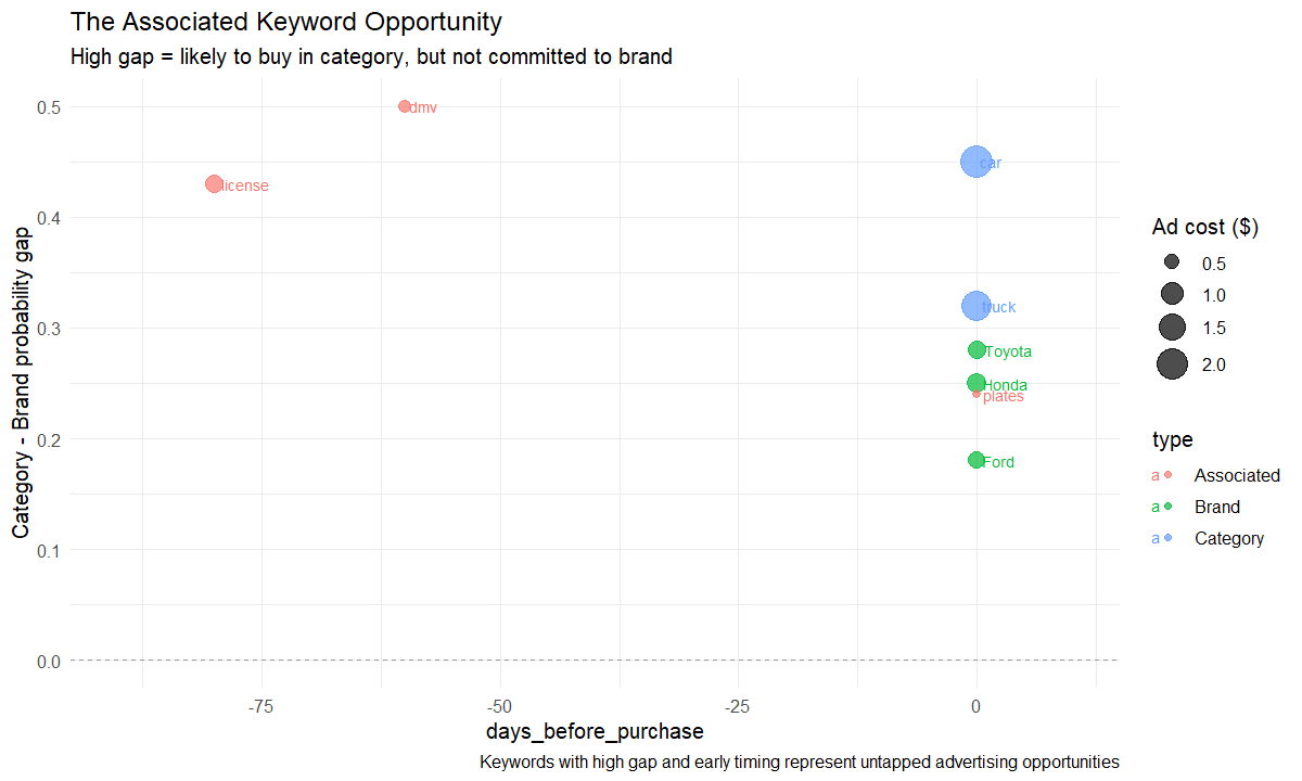
The plot shows what the paper describes: associated keywords like “license,” “battery,” and “dmv” appear early in the journey (negative days), have a high gap between category and brand probability, and cost significantly less than category terms.
Model accuracy with search history
The paper shows that just 5 days of search history dramatically improves prediction accuracy. Let me simulate this:
# Diminishing returns model based on paper's findings
days_history <- c(0, 1, 2, 3, 5, 7, 14, 30, 60, 90)
base_accuracy <- 0.65
max_improvement <- 0.15  # 8-15 pp improvement from paper

accuracy_fn <- function(days) {
  base_accuracy + max_improvement * (1 - exp(-0.3 * days))
}

model_accuracy <- data.frame(
  days_history = days_history,
  accuracy = sapply(days_history, accuracy_fn)
)

ggplot(model_accuracy, aes(x = days_history, y = accuracy)) +
  geom_line(color = "#1f77b4", linewidth = 1.2) +
  geom_point(color = "#1f77b4", size = 3) +
  geom_vline(xintercept = 5, linetype = "dashed", color = "gray50") +
  annotate("text", x = 5, y = 0.68, label = "5 days: ~85% of max benefit",
           hjust = 1.1, vjust = 0, size = 3, color = "gray50") +
  scale_x_continuous("Days of search history considered") +
  scale_y_continuous("Model accuracy in predicting conversion",
                    labels = scales::percent, limits = c(0.60, 0.85)) +
  labs(title = "Prediction Accuracy Improves with Search History",
       subtitle = "Diminishing returns after ~5-7 days of context") +
  theme_minimal(base_size = 12)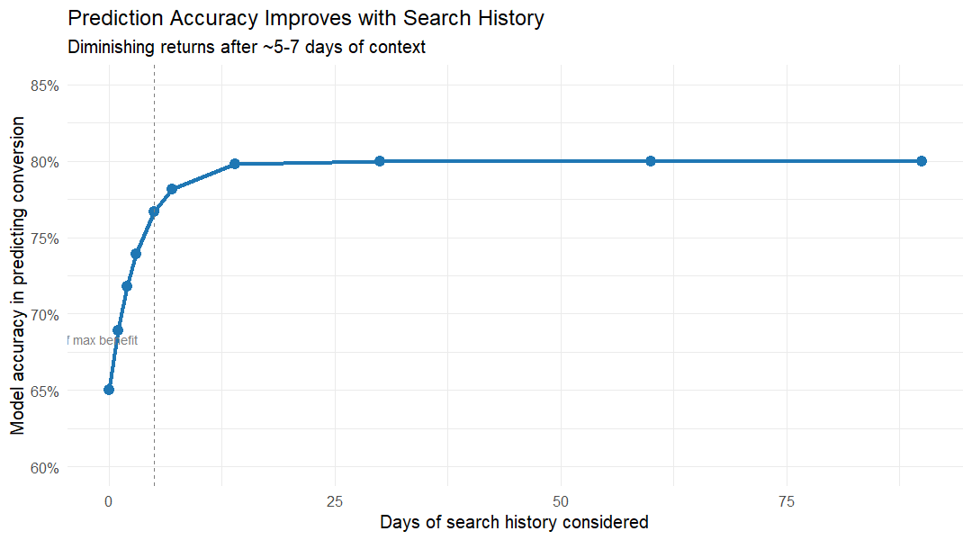
The key insight here is that most of the benefit comes from just a few days of context. After about 7 days, additional history provides minimal additional value.
Ad lift by journey stage
# Simulated ad lift by keyword type and journey stage
# Based on patterns described in the paper

journey_stage <- c("Early (>45 days)", "Mid (15-45 days)", "Late (<15 days)", "At purchase")
ad_lift_by_stage <- data.frame(
  stage = journey_stage,
  brand_keywords = c(1.15, 1.30, 1.45, 1.50),
  category_keywords = c(1.05, 1.12, 1.25, 1.35),
  associated_keywords = c(1.20, 1.18, 1.10, 1.05)
)

p4_long <- ad_lift_by_stage %>%
  tidyr::pivot_longer(cols = c(brand_keywords, category_keywords, associated_keywords),
                     names_to = "keyword_type",
                     values_to = "lift") %>%
  mutate(keyword_type = factor(keyword_type,
                            levels = c("associated_keywords", "category_keywords", "brand_keywords"),
                            labels = c("Associated", "Category", "Brand")),
         stage = factor(stage, levels = c("Early (>45 days)", "Mid (15-45 days)", "Late (<15 days)", "At purchase")))

ggplot(p4_long, aes(x = stage, y = lift, fill = keyword_type, group = keyword_type)) +
  geom_line(linewidth = 0.8) +
  geom_point(size = 3.5, shape = 21, color = "white", stroke = 1.5) +
  geom_hline(yintercept = 1.0, linetype = "dashed", color = "gray60") +
  scale_y_continuous("Conversion lift multiplier", breaks = seq(1.0, 1.6, 0.1)) +
  scale_fill_manual("Keyword type", values = c("#2ca02c", "#ff7f0e", "#1f77b4")) +
  labs(title = "Ad Lift Varies by Keyword Type and Journey Stage",
       subtitle = "Brand keywords strongest at purchase; Associated keywords valuable early") +
  theme_minimal(base_size = 12) +
  theme(axis.text.x = element_text(angle = 45, hjust = 1),
        legend.position = "bottom")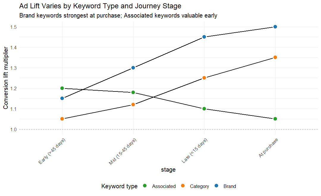
The pattern here shows that brand keywords work best at the point of purchase, but associated keywords provide meaningful lift earlier in the journey when the customer is still undecided about the brand.
Implications for LLM-based search
The paper ends with an interesting observation: as search moves toward LLM-based conversational interfaces, platforms will have more context than just a single query. Multistage conversations will provide rich signals about where a user is in their conversion journey.
This could change the advertising landscape significantly. If the platform can understand context from a conversation rather than just a keyword, the entire targeting model shifts from “who searched for X” to “who is in stage Y of their journey for product category Z.”
Limitations
The paper acknowledges several limitations: it uses observational and natural experiments rather than RCTs, focuses on three product categories that are purchased multiple times over a lifetime, and analyzes data from Bing (which has smaller market share than Google).
My simulation has additional limitations: it’s based on published summary statistics rather than raw data, and the ad lift by stage is illustrative rather than directly estimated from the paper.
Takeaways
The most useful insight for me is the “commitment gap” — identifying users who are committed to buying in the category but not yet committed to a brand. This is where associated keywords provide the most value, and it’s where advertisers currently spend the least.
If you are running search campaigns, consider:
- Identifying associated keywords in your category
- Testing their cost-effectiveness early in the funnel
- Using minimal search history (5-7 days) to improve targeting without significant privacy cost