tfestimators - Package: Embeddings for Categorical Variables
In my last posts (here and here) I explored how to use embeddings to represent categorical variables. Furthermore, I showed how to represent categorical variables with embeddings and add other variable to create a more complex model. Both posts focused on the Keras (R) functionality. I concluded that it feels artificial to represent categorical variables with embeddings in Keras. Especially concatenating multiple input layers is quite cumbersome with the current Keras interface.
This week, I watched the official release video by J.J. Allaire and learnt about the tfestimators package. It turns out that the awesome rstudio team build a very handy interface to access tensorflow and train models with multiple parameters and embeddings.
In this post, I will show how to use the package to quickly fit a model in which categorical variables are represented as embeddings.
As in the posts before, I work with the nyc citi bike count data from Kaggle. It contains daily bicycle counts for 4 major bridges in NYC. In order to have a longer dataset, I use the bicycle count for all bridges as the dependent variable.
#https://www.kaggle.com/new-york-city/nyc-east-river-bicycle-crossings
df <- read.csv("data/nyc-east-river-bicycle-counts.csv")

dflong <- data.table::melt(df[c("Date", "Brooklyn.Bridge", "Manhattan.Bridge", "Williamsburg.Bridge" ,"Queensboro.Bridge")], idvars="date")

dflong$date <- as.Date(dflong$Date)
dflong$weekday <- wday(dflong$date, label = T)

dflong <- merge(dflong, df[, c("Date", "Precipitation", "Low.Temp..Â.F.")], by="Date")

dflong$ScaledUsers <- scale(dflong$value)
dflong$lowTemp <- scale(dflong[,"Low.Temp..Â.F."])

dflong$rain <- ifelse(dflong$Precipitation != 0, 0,1)

dflong$Bridge <- factor(dflong$variable)
levels(dflong$Bridge) <- 1:length(levels(dflong$Bridge))
levels(dflong$weekday) <- 1:length(levels(dflong$weekday))
The goal of our play model is to predict the number of bicycle per day on a certain bridge dependent on the weekday, the bridge (“Brooklyn.Bridge”, “Manhattan.Bridge”, “Williamsburg.Bridge” ,”Queensboro.Bridge”), if it rains and the temperature. So overall we have 2 categorical variables, one binary and one continuous variable.
library(tfestimators)

## convert the factor to integer -- tfestimators is strict with input types.
dflong$Bridge <- as.integer(dflong$Bridge)
dflong$weekday <- as.integer(dflong$weekday)

embedding_dimension_bridges = 2
embedding_dimension_weekdays = 3

cols <- feature_columns(
  column_numeric("lowTemp","rain"),

  column_embedding(column_categorical_with_vocabulary_list("weekday", vocabulary_list = c(1:7)), embedding_dimension_weekdays),
  column_embedding(column_categorical_with_vocabulary_list("Bridge",vocabulary_list = c(1:4)), embedding_dimension_bridges)
)
The first step that we need to do is to define the input variables and their type. Let’s start with the simple numeric variables lowTemp and rain. We just define the input as “column_numeric(“lowTemp”,”rain”)”. Next, the two categorical variables that we want to embed, need a bit more work. a) they need a list of all possible values (defined in vocabulary_list parameter). Additionally, we need to define the embedding_dimension for each categorical variable.
Next, we write a short function that defines the input and output of the the model as well as batch size and number of epochs.
library(tfestimators)

bridge_input_fn <- function(data, num_epochs = 1) {
  tfestimators::input_fn(data,
           features = c("lowTemp","rain","weekday", "Bridge"),
           response = "ScaledUsers",
           batch_size = 2,
           num_epochs = num_epochs)
}

############ Train and Test Dataset #############

indices <- sample(1:nrow(dflong), size = 0.80 * nrow(dflong))
train <- dflong[indices, ]
test  <- dflong[-indices, ]

############## Define the model ############
model <- dnn_regressor(feature_columns = cols, hidden_units = c(32, 10), dropout = 0.15)

# train the model
history <- model %>% train(bridge_input_fn(train[,c("ScaledUsers", "lowTemp","rain","weekday", "Bridge" )], num_epochs = 1))

## eval the output
model %>% evaluate(bridge_input_fn(test))
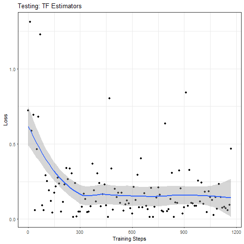
In order to evaluate the model, we split the data in train and test set. We define the model as deep neural network (DNN), regression model with two hidden layers (one with 32 the other with 10 nodes). Compared to the Keras version, in which one needs to concatenate different input layers this interface is straight-forward. Finally, we check the model’s accuracy on test set and print the learning history.
require(ggplot2)
df <- data.frame(losses = history$losses$mean_losses, steps=history$step)
ggplot(df, aes(steps, losses))+ geom_point() +geom_smooth() +theme_bw() + ylab("Loss") + xlab("Training Steps") + ggtitle("Testing: TF Estimators")
To conclude, the package is a great step forward to apply deep neural nets to everyday problems and to quickly use embeddings for categorical variables. Big Kudus to the Rstudio team for their efforts. If you have time left and want a quick update on deep learning for the R community check out J.J. Allaire’s video.