Concatenate Embeddings for Categorical Variables with Keras
In my last post, I explored how to use embeddings to represent categorical variables. Furthermore, I showed how to extract the embeddings weights to use them in another model.
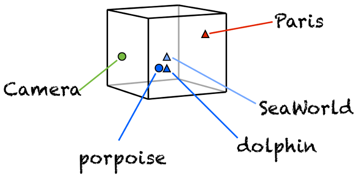
While the concept of embedding representation has been used in NLP for quite some time, the idea to represent categorical variables with embeddings appreared just recently If you are interested in learning more about embddings, this is a good resource for the concept. The image (from quora) quickly summarises the embedding concept. Words or categorical variables are represented by a point in n or in this case 3-dimensional space. Words which are similar are grouped together in the cube at a similar place.
In response to my post, I got the question of how to combine such embeddings with other variables to build a model with multiple variables. This is a good question and not straight-forward to achieve as the model structure inn Keras is slightly different from the typical sequential model.
As in the post before, let’s work with the nyc citi bike count data from Kaggle. It contains daily bicycle counts for major bridges in NYC.
In order to have a longer dataset, I use the bicycle count for all bridges as the dependent variable
#https://www.kaggle.com/new-york-city/nyc-east-river-bicycle-crossings
df <- read.csv("data/nyc-east-river-bicycle-counts.csv")


dflong <- data.table::melt(df[c("Date", "Brooklyn.Bridge", "Manhattan.Bridge", "Williamsburg.Bridge" ,"Queensboro.Bridge")], idvars="date")

dflong$date <- as.Date(dflong$Date)
dflong$weekday <- wday(dflong$date)

dflong <- merge(dflong, df[, c("Date", "Precipitation", "Low.Temp..Â.F.")], by="Date")

dflong$ScaledUsers <- scale(dflong$value)
dflong$lowTemp <- scale(dflong[,"Low.Temp..Â.F."])

dflong$rain <- ifelse(dflong$Precipitation != 0, 0,1)

### important - replace string factors with numbers for Keras to work!
dflong$Bridge <- factor(dflong$variable)
levels(dflong$Bridge) <- 1:length(levels(dflong$Bridge))
Please note the code last lines. Keras works only with double and integer variables, hence we have to replace the Bridge-factor variable with indicies between 1 and 4. The goal of our play model is to predict the number of bicycle per day on a certain bridge dependent on the weekday, the bridge (“Brooklyn.Bridge”, “Manhattan.Bridge”, “Williamsburg.Bridge” ,”Queensboro.Bridge”), if it rains and the temperature. So overall we have 2 categorical variables, one binary and one continuous variable.
One simple way to use a deep net with this dataset is to “One-hot” encode the categorical variables, combine them in one dataframe.
require(keras)

dfOneHot <- data.frame(to_categorical(dflong$weekday, 8), to_categorical(dflong$Bridge, 5), dflong$rain, dflong$lowTemp)

model_simple <- keras_model_sequential()

model_simple %>%
  layer_dense(input_shape=(8+5+1+1), units=32, activation = "relu") %>%
  layer_dropout(0.4) %>%
  layer_dense(units=10, activation = "relu") %>%
  layer_dropout(0.2) %>%
  layer_dense(units=1)


model_simple %>% compile(loss = "mean_squared_error", optimizer = "sgd", metric="accuracy")

model_simple %>% fit(x = as.matrix(dfOneHot), y= as.matrix(dflong$ScaledUsers), epochs = 20, batch_size = 5, validation_split = 0.15)
Pretty straight-forward and the only points where people struggle is; setting the input correct (15) and to remember that we need to cast the dataframe to a matrix. So what about using embeddings instead of one-hot encodings? How can we combine two embeddings (weekday and bridge) with a binary (rain/no-rain) and continuous variable (temperature)?
First we define 3 input layers, one for every embedding and one the two variables. As both categorical variables are just a vector of lenght 1 the shape=1. For the last layer where we feed in the two other variables we need a shape of 2.
Next, we create the two embedding layer. The input dimension is the number of unique values +1, for the dimension we use last week’s rule of thumb.
Third, we concatenate the 3 layers and add the network’s structure. Finally, we use the keras_model (not keras_sequential_model) to set create the model.
embedding_size_weekday=3
embedding_size_bridge=2

## 1
inp1 <- layer_input(shape = c(1), name = 'inp_weekday')
inp2 <- layer_input(shape = c(1), name = 'inp_bridge')
inp3 <- layer_input(shape = c(2), name = 'inp_otherVars')

## 2
embedding_out1 <- inp1 %>% layer_embedding(input_dim = 7+1, output_dim = embedding_size_weekday, input_length = 1, name="embedding_weekday") %>%  layer_flatten()

embedding_out2 <- inp2 %>% layer_embedding(input_dim = 4+1, output_dim = embedding_size_bridge, input_length = 1, name="embedding_bridge") %>%  layer_flatten()

## 3
combined_model <- layer_concatenate(c(embedding_out1, embedding_out2, inp3)) %>%
  layer_dense(units=32, activation = "relu") %>%
  layer_dropout(0.3) %>%
  layer_dense(units=10, activation = "relu") %>%
  layer_dropout(0.15) %>%
  layer_dense(units=1)

## 4
model <- keras::keras_model(inputs = c(inp1, inp2, inp3), outputs = combined_model)

model %>% compile(loss = "mean_squared_error", optimizer = "sgd", metric="accuracy")

summary(model)
## ___________________________________________________________________________
## Layer (type) Output Shape Param # Connected to
## ===========================================================================
## inp_weekday (InputLayer (None, 1) 0
## ___________________________________________________________________________
## inp_bridge (InputLayer) (None, 1) 0
## ___________________________________________________________________________
## embedding_weekday (Embe (None, 1, 3) 24 inp_weekday[0][0]
## ___________________________________________________________________________
## embedding_bridge (Embed (None, 1, 2) 10 inp_bridge[0][0]
## ___________________________________________________________________________
## flatten_35 (Flatten) (None, 3) 0 embedding_weekday[0][0]
## ___________________________________________________________________________
## flatten_36 (Flatten) (None, 2) 0 embedding_bridge[0][0]
## ___________________________________________________________________________
## inp_otherVars (InputLay (None, 2) 0
## ___________________________________________________________________________
## concatenate_29 (Concate (None, 7) 0 flatten_35[0][0]
## flatten_36[0][0]
## inp_otherVars[0][0]
## ___________________________________________________________________________
## dense_126 (Dense) (None, 32) 256 concatenate_29[0][0]
## ___________________________________________________________________________
## dropout_33 (Dropout) (None, 32) 0 dense_126[0][0]
## ___________________________________________________________________________
## dense_127 (Dense) (None, 10) 330 dropout_33[0][0]
## ___________________________________________________________________________
## dropout_34 (Dropout) (None, 10) 0 dense_127[0][0]
## ___________________________________________________________________________
## dense_128 (Dense) (None, 1) 11 dropout_34[0][0]
## ===========================================================================
## Total params: 631
## Trainable params: 631
## Non-trainable params: 0
## ___________________________________________________________________________The model summary shows that the input takes place at different times during training. The input of the “other” variables happens late in the process.
In order to train this model, we need to feed the data in a list structure. Each input layer gets their own list of elements.
### a list with an element for each individual input layer.
inputVariables <- list(as.matrix(dflong$weekday), as.matrix(dflong$Bridge), as.matrix(dflong[,c("lowTemp","rain")]))

model %>% fit(x = inputVariables,
              y= as.matrix(dflong$ScaledUsers), epochs = 20, batch_size = 2)
Comparing the two approaches, it is pretty clear that the one-hot encoding will stay the norm. It feels very artificial to represent categorical variables with embeddings in Keras. There is either room for a wrapper function to automatically create the input layer part or a redesign of layer_concatenate function.