Transfer Learning with Keras in R
In my last posts ([here](http://flovv.github.io/Logo_detection_deep_learning/ and here, I described how one can detect logos in images with R. The first results were promising and achieved a classification accuracy of ~50%. In this post i will detail how to do transfer learning (using a pre-trained network) to further improve the classification accuracy.
The dataset is a combination of the Flickr27-dataset, with 270 images of 27 classes and self-scraped images from google image search. In case you want to reproduce the analysis, you can download the set here.
In addition to the previous post, this time I wanted to use pre-trained image models, to see how they perform on the task of identifing brand logos in images. First, I tried to adapt the official example on the Keras-rstudio website.
Here is a copy of the instructions:
# create the base pre-trained model
base_model <- application_inception_v3(weights = 'imagenet', include_top = FALSE)

# add our custom layers
predictions <- base_model$output %>%
  layer_global_average_pooling_2d() %>%
  layer_dense(units = 1024, activation = 'relu') %>%
  layer_dense(units = 200, activation = 'softmax')

# this is the model we will train
model <- keras_model(inputs = base_model$input, outputs = predictions)

# first: train only the top layers (which were randomly initialized)
# i.e. freeze all convolutional InceptionV3 layers
for (layer in base_model$layers)
  layer$trainable <- FALSE

# compile the model (should be done *after* setting layers to non-trainable)
model %>% compile(optimizer = 'rmsprop', loss = 'categorical_crossentropy')

# train the model on the new data for a few epochs
model %>% fit_generator(...)

# at this point, the top layers are well trained and we can start fine-tuning
# convolutional layers from inception V3. We will freeze the bottom N layers
# and train the remaining top layers.

# let's visualize layer names and layer indices to see how many layers
# we should freeze:
layers <- base_model$layers
for (i in 1:length(layers))
  cat(i, layers[[i]]$name, "\n")

# we chose to train the top 2 inception blocks, i.e. we will freeze
# the first 172 layers and unfreeze the rest:
for (i in 1:172)
  layers[[i]]$trainable <- FALSE
for (i in 173:length(layers))
  layers[[i]]$trainable <- TRUE

# we need to recompile the model for these modifications to take effect
# we use SGD with a low learning rate
model %>% compile(
  optimizer = optimizer_sgd(lr = 0.0001, momentum = 0.9),
  loss = 'categorical_crossentropy'
)

# we train our model again (this time fine-tuning the top 2 inception blocks
# alongside the top Dense layers
model %>% fit_generator(...)
It is basically a three step process; 1) load an existing model and add some layers, 2) train the extended model on your own data, 3) set more layers trainable and fine-tune the model on your own data.
I have to admit that I struggled to make it work on my data. That’s why I will try to detail my approach. Hopefully it helps you to get better started with transfer learning.
Here is the full example that I got to work:
require(keras)
### Keras transfer learning example

################### Section 1 #########################
img_width <- 32
img_height <- 32
batch_size <- 8

train_directory <- "flickrData/train"
test_directory <- "flickrData/test"

train_generator <- flow_images_from_directory(train_directory, generator = image_data_generator(),
                                              target_size = c(img_width, img_height), color_mode = "rgb",
                                              class_mode = "categorical", batch_size = batch_size, shuffle = TRUE,
                                              seed = 123)

validation_generator <- flow_images_from_directory(test_directory, generator = image_data_generator(),
                                                   target_size = c(img_width, img_height), color_mode = "rgb", classes = NULL,
                                                   class_mode = "categorical", batch_size = batch_size, shuffle = TRUE,
                                                   seed = 123)
train_samples = 498
validation_samples = 177

################### Section 2 #########################
#base_model <- application_inception_v3(weights = 'imagenet', include_top = FALSE)
base_model <- application_vgg16(weights = 'imagenet', include_top = FALSE)
### use vgg16 -  as inception won't converge ---

################### Section 3 #########################
## add your custom layers
predictions <- base_model$output %>%
  layer_global_average_pooling_2d(trainable = T) %>%
  layer_dense(64, trainable = T) %>%
  layer_activation("relu", trainable = T) %>%
  layer_dropout(0.4, trainable = T) %>%
  layer_dense(27, trainable=T) %>%    ## important to adapt to fit the 27 classes in the dataset!
  layer_activation("softmax", trainable=T)
# this is the model we will train
model <- keras_model(inputs = base_model$input, outputs = predictions)

################### Section 4 #########################
for (layer in base_model$layers)
  layer$trainable <- FALSE

################### Section 5 #########################
model %>% compile(
  loss = "categorical_crossentropy",
  optimizer = optimizer_rmsprop(lr = 0.003, decay = 1e-6),  ## play with the learning rate
  metrics = "accuracy"
)

hist <- model %>% fit_generator(
  train_generator,
  steps_per_epoch = as.integer(train_samples/batch_size),
  epochs = 20,
  validation_data = validation_generator,
  validation_steps = as.integer(validation_samples/batch_size),
  verbose=2
)

### saveable data frame obejct.
histDF <- data.frame(acc = unlist(hist$history$acc), val_acc=unlist(hist$history$val_acc), val_loss = unlist(hist$history$val_loss),loss = unlist(hist$history$loss))
The key change to the Rstudio sample code is to use a different pre-trained model. I use VGG16 over Inception_v3 as the later would work. (The Inception-model would not pick up any information and accuracy remains around the base rate.) But let’s see what the code does step by step. In section 1 the image data is prepared and loaded. One that setting that is important to set while loading the images is “class_mode = “categorical””, as we have 27 different image classes/labels to assign. In section 2 we load the pretrained image model. In section 3 we add custom layers. (In this case I copied the last layers from the previous post.) It is important to set the last layers to the number of labels (27) and the activation function to softmax. In section 4 we set the layers of the loaded image model to non-trainable. Section 5 sets the optimiser and finally trains the model. If the training process does not show improvements in terms of decreasing loss, try to increase the learning rate. The learning process is documented in the hist-object, which can be easily plotted.
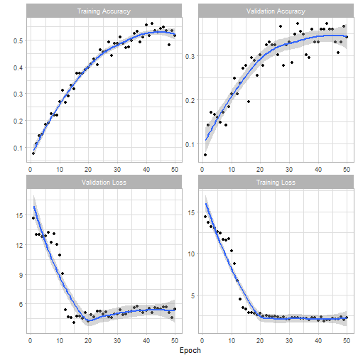
After 50 Traing-epochs the accuracy is at 55% on the training 35% on the validation set. I assume that the accuracy can be further improved by training the full model or at least set more layers trainable and fine tune the full model as it is detailed in the R-Studio case. However, so far I tried various parameter settings without success. There is basically no improvement on the established 50%, yet.
I will update the post, as soon as I have figured it out.