Predominately data science projects deal with descriptive statistics. The common theme (especially on this blog) is to gather a dataset, visualize and describe it. The toolset consists of a combination of machine learning, descriptive statistics and (gg-)plots. This time I want to go a step further; from descriptive to prescriptive analytics. The goal is to optimize a fantasy football team. To be more precise the task at hand is to select a set of players while keeping within the budget (e.g. a typical knapsack problem). For that I first gathered some fantasy football data from comunio.de

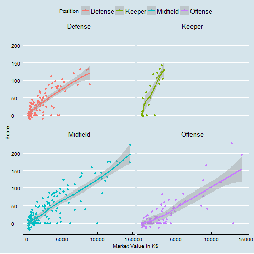
The plot above nicely illustrates the data. It basically contains of a list of players (488) which hold one of four positions and are characterized by two basic variables; (a) the market value, - for how much a player can be bought on the fantasy market, and (b) the Score which indicates how well a player has performed.

A simple optimization problem is to figure out how to maximize the number of points while keeping within the team budget. There are two more constraints on the line-up, each team needs to have exactly one keeper and a dynamic number of players on the defense, midfield and offensive positions. As players might be injured during the season, let’s simplify the line-up constraints and the maximum for each position is 1 keeper, 5 defender, 5 midfielder and 3 scorer. Additionally, in total a team consists of exactly 13 players.

How can we setup this optimization problem in R? In contrast to most formal definitions, I will start defining the solution backwards.

First, let’s define the objective; it is to maximize team score. The decision is which player to pick to maximize the score. Hence the decision variables (x1 - x488) are binary and are multiplied with the individual player score. The “simple” dataframe contains all players with their market value, score and position. In order to setup the objective vector I simply take the “Score” vector. Then I define the right-hand side of the constraints using two vectors. It is important that the positions align (e.g. the 1 refers to the keeper position which should equal.)

library(lpSolve)
 
f.obj <- simple$Score  ### objective! 
 
## constraints 
#budget 20 mio, 13 players, 1 keeper, 5 defender, ... 3 scorer
f.rhs <- c(20000000, 13, 1, 5, 5, 3)
#coresponding budget needs to lower than defined above, exactly 1 keeper
f.dir <- c("<=", "<=", "=", "<=", "<=" ,"<=")

Next I need to setup the left-hand side accordingly. In order to keep the right order (matching the left hand side), I start with the market value of each player. The sum over the decision variables times the individual market value should be lower than 20 Million. Than I define a player vector set to 1 equal to the size of the dataframe.

f.con <- t(simple$MarketValue)  ### constraints max MV <= Budget
player <- rep(1, nrow(simple))  ## constraints max number of players!
f.con <- rbind(f.con, player)

Finally, for the left-hand side, I need to take into consideration the position each player holds. A nice function allows to one-hot encode the dummy “Position” variable in a suitable matrix.

## constrain that per postion can only be a certain number of players be set up. (e.g. just one keeper)
## define matrix   - as a one hot (dummy coding what position the player holds)
A <- as.data.frame(model.matrix(MarketValue ~ Position -1, simple) )
f.con <- rbind(f.con, t(as.matrix(A)))

That brings us to the nice part: solving the linear program using lpsolve. The solution represents the decision variables, indicating which of the player should be bought. Applying that back to the dataframe, I get the optimal score, market value and the name of players to be bought.

### solve the problem
solved<- lp("max", f.obj, f.con, f.dir, f.rhs, all.bin=TRUE)  ## just binary decision variables!
 
###################output!
simple$buy <- solved$solution
 
sum(out[out$buy == 1,]$MarketValue)  ## what is the Budget

## [1] 19800000

sum(out[out$buy == 1,]$Score) ## what is the Score

## [1] 784

sum(out[out$buy == 1,]$buy)   ## number of players bought

## [1] 13

paste(out[out$buy == 1,]$Name, collapse=", ")  

## [1] "Badstuber, Baier, Balitsch, Ede, Gomez, Hasebe, Klavan, Krmas, Piszczek, R. Schäfer, Soto, Svensson, Werner"

That’s it. Instead of just describing the dataset and figuring out which players performed well according to some metric, I used just ~40 lines of code to get the optimal result while keeping within the constraints. On a general note; while these problems are pretty common in various industries, the problem class and solution is vastly undervalued by data scientists and online courses.

Well ordered source code: