In order to stay up to date, I try to follow Jeremy Howard on a regular basis. In one of his recent videos, he shows how to use embeddings for categorical variables (e.g. weekdays).

First off; what are embeddings? An embedding is a mapping of a categorical vector in a continuous n-dimensional space. The idea is to represent a categorical representation with n-continuous variables. To make it more concrete, let’s say you want to model the effect of day of the week on an outcome. Usually you would try to one-hot encode the variable, which means that you create 6 variables (each for one day of a week minus 1) and set the variable 1 or 0 depending on the value. You end up having a 6-dimensional space to represent a weekday.
So, what is the advantage of mapping the variables in an continuous space? In a nutshell; with embeddings you can reduce the dimensionality of your feature space which should reduce overfitting in prediction problems.

In order to test the idea on a play example, I downloaded the nyc citi bike count data from Kaggle. It contains daily bicycle counts for major bridges in NYC.

#https://www.kaggle.com/new-york-city/nyc-east-river-bicycle-crossings
df <- read.csv("data/nyc-east-river-bicycle-counts.csv")
 
df$date <- as.Date(df$Date)
df$weekday <- lubridate::wday(df$date)
df$users <- df$Brooklyn.Bridge
 
df <- df[df$users>0,]
df <- df[!is.na(df$users),]
df <- df[!is.na(df$weekday),]
 
df$ScaledUsers <- scale(df$users)

Next, we set up a sequentual model with keras. The first layer is the embedding layer with the size of 7 weekdays plus 1 (for the unknowns). The embedding-size defines the dimensionality in which we map the categorical variables. Jeremy Howard provides the following rule of thumb; embedding size = min(50, number of categories/2).

require(keras)
embedding_size <- 3

model <- keras_model_sequential()

model %>% layer_embedding(input_dim = 7+1, output_dim = embedding_size, input_length = 1, name="embedding") %>%
  layer_flatten()  %>%  
  layer_dense(units=40, activation = "relu") %>%  
  layer_dense(units=10, activation = "relu") %>%  
  layer_dense(units=1)

model %>% compile(loss = "mse", optimizer = "sgd", metric="accuracy")

hist <- model %>% fit(x = as.matrix(df$weekday), y= as.matrix(df$ScaledUsers), epochs = 50, batch_size = 2)

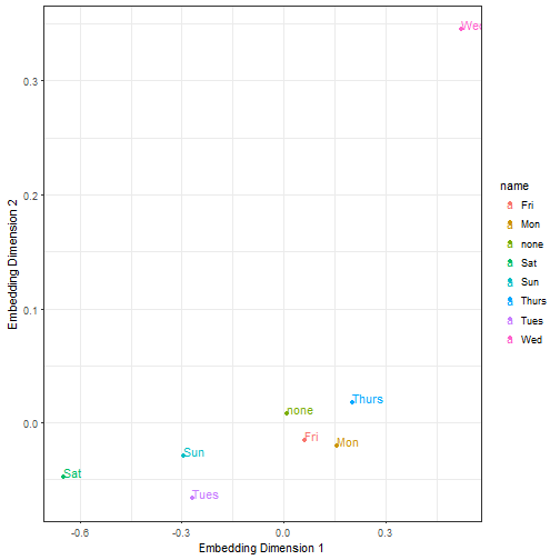
It is important to have a rather small batch size and to scale the count data. After training the model, we can extract individual layers. We named the first layer “embedding”. The weights of the embedding layer define where in the 3-dimensional feature space the network has placed the variables. We can show that by plotting the points in a scatterplot.

layer <- get_layer(model, "embedding")
 
embeddings <- data.frame(layer$get_weights()[[1]])
embeddings$name <- c("none", levels(wday(df$date, label = T)) )
 
ggplot(embeddings, aes(X1, X2, color=name))+ geom_point() +geom_text(aes(label=name),hjust=0, vjust=0) + theme_bw() + xlab("Embedding Dimension 1") +ylab("Embedding Dimension 2")

The great thing about the embedding layer weights are, that they act as a lookup table. Merging the variables back to our dataset we can use the dimensions as input (X1, X2, X3) for a simple linear regression replacing the categorical representation of the day of the week variable.

df$weekDayF <- wday(df$date, label = T)
embeddings$lookup <- c("none", levels(df$weekDayF))
dff <- merge(df, embeddings, by.x="weekDayF", "lookup")
 
## we trained the embeddings on the Brooklyn.Bridge variable but test it on another ...
dff$users <- dff$Manhattan.Bridge
 
testRun <- function(x){
    sample <- caret::createDataPartition(dff$weekDayF, list=FALSE, p = 0.8)
    train <- dff[sample,]
    test <- dff[-sample,]
    
    fit1 <- lm(users ~ X1 + X2 + X3, data=train)
    fit2 <- lm(users ~ weekDayF  , data=train)   # 6 input variables as lm automatically one-hot encodes categorical variables.
    
   data.frame(run=x,
     Embedding=sqrt(mean((predict(fit1, test) - test$users)^2)), 
     Categorical=sqrt(mean((predict(fit2, test) - test$users)^2) ))
}
 
test <- plyr::ldply(1:100, function(x){testRun(x)})
mm <- data.table::melt(test, id.vars="run")
dd <- plyr::ddply(mm,.(variable), summarise, m=mean(value))
 
df2 <- Rmisc::summarySE(mm, "value", "variable")
ggplot(df2, aes(x=variable, y=value)) + 
  geom_point()+
  geom_errorbar(aes(ymin=value-se, ymax=value+se), width=.2,
                 position=position_dodge(0.05)) +ylab("Mean Error") + xlab("Regression Input") + theme_bw()

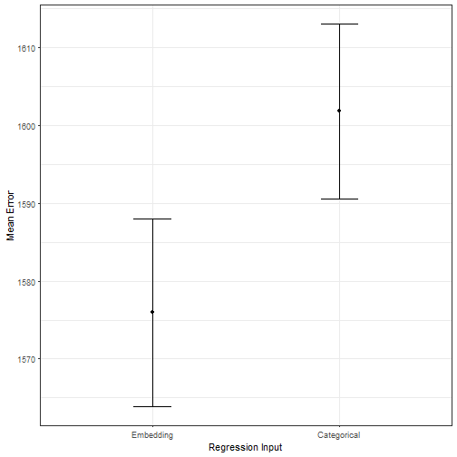
Further, we can test if the embedding model outperforms the categorical regression model in an out of sample evaluation. The plot above shows the mean error over 100 test-runs (training on 80%, testing on 20%, metric: RMSE.) The embedding model (with a more compact representation of the day of the week) outperforms the categorical model.

I expect to see more data scientists using embeddings for categorical variables in the upcoming years for prediction problems. While the mapping reduces interpretability, it apparently helps to find a better prediction model. This has also been shown by Cheng Guo and Felix Berkhahn. They note: “embeddings help to generalize better when the data is sparse and statistics is unknown. Thus, it is especially useful for datasets with lots of high cardinality features, where other methods tend to overfit.”

In a follow up post, I will try to transfer learn such embeddings. The idea is to learn a (weekday) embedding on one problem and transfer it to a different dataset.