Analyzing "Call a Bike" bike sharing data.
Call a bike is a service of the “Deutsche Bahn”, providing a rental bikes for short trips similar to citibikeNYC. I used it extensively for some time. Recently I found out that they provide individual trip data trough their API. I pulled last year’s data from the “CallaBike”-SOAP API.
So it looks like I did 403 trips using a Call a Bike in 2014.
After some data cleaning, we will take an initial glimpse at the data.

We see a clear pattern of high usage during the week and at commuting hours.
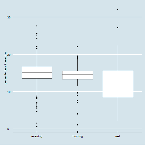
Commute times are basically the same for the morning/evening trips.
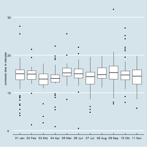
Commute times did not change over the year. (some ups and downs -but it’s basically stable.)
According to Google Maps the distance is 4.9km. Which makes a total of 1969.8 KM in 2014, at an average speed of: 20.45.
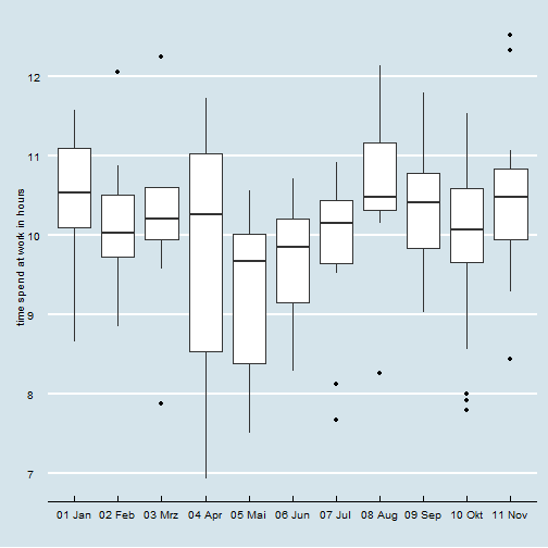
As this data indicates starting and ending of commutes, we can calculate the time spend at work.
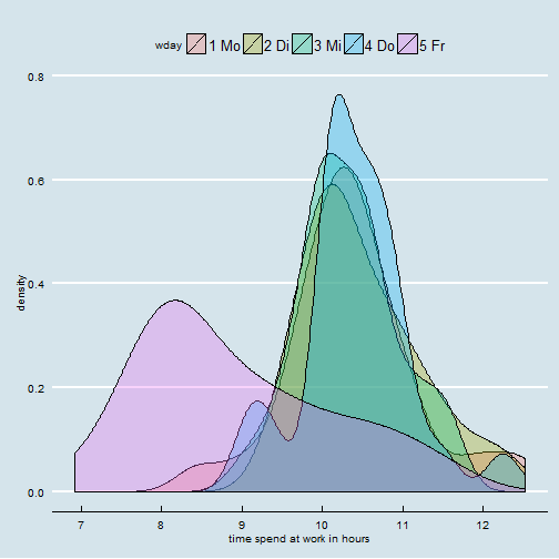
Looks like an easy 50.512 hours week (on average). With the time spend at work being quite similar from Monday till Tuesday, and Fridays being more relaxed.
And finally some regression model (using the fantastic stargazer package) to explain the time spend at work …
lm <- lm(wt~wday+mon+dt.x+dt.y, data=working)
lm1 <- lm(wt~wday+mon, data=working)

stargazer(lm1, lm, type = "html", title="Explaining time spend at work.")| Dependent variable: | ||
| wt | ||
| (1) | (2) | |
| wday2 Di | 0.154 | 0.115 |
| (0.188) | (0.186) | |
| wday3 Mi | 0.022 | 0.004 |
| (0.190) | (0.186) | |
| wday4 Do | 0.108 | 0.144 |
| (0.204) | (0.200) | |
| wday5 Fr | -1.499*** | -1.536*** |
| (0.197) | (0.193) | |
| mon02 Feb | -0.726** | -0.775*** |
| (0.284) | (0.279) | |
| mon03 Mrz | -0.613** | -0.680** |
| (0.302) | (0.296) | |
| mon04 Apr | -0.842*** | -0.930*** |
| (0.261) | (0.258) | |
| mon05 Mai | -1.369*** | -1.303*** |
| (0.290) | (0.286) | |
| mon06 Jun | -1.260*** | -1.262*** |
| (0.254) | (0.250) | |
| mon07 Jul | -0.858*** | -0.947*** |
| (0.234) | (0.234) | |
| mon08 Aug | -0.395 | -0.406 |
| (0.286) | (0.280) | |
| mon09 Sep | -0.600** | -0.585** |
| (0.296) | (0.290) | |
| mon10 Okt | -0.922*** | -0.894*** |
| (0.237) | (0.233) | |
| mon11 Nov | -0.559** | -0.656*** |
| (0.251) | (0.250) | |
| dt.x | -0.037 | |
| (0.025) | ||
| dt.y | -0.041** | |
| (0.016) | ||
| Constant | 11.071*** | 12.252*** |
| (0.213) | (0.487) | |
| Observations | 161 | 161 |
| R2 | 0.491 | 0.520 |
| Adjusted R2 | 0.442 | 0.466 |
| Residual Std. Error | 0.759 (df = 146) | 0.743 (df = 144) |
| F Statistic | 10.069*** (df = 14; 146) | 9.743*** (df = 16; 144) |
| Note: | *p<0.1; **p<0.05; ***p<0.01 | |
Why is time spend at work negatively correlated with drive time back from work (variable dt.y)? Finally 3 models to explain the commute time back from work.
lm3 <- lm(dt.y~wt, data=working)
lm4 <- lm(dt.y~wt+wday, data=working)
lm5 <- lm(dt.y~wt+wday +mon, data=working)

stargazer(lm3,lm4,lm5, type = "html", title="Explaining commute time back from work.")| Dependent variable: | |||
| dt.y | |||
| (1) | (2) | (3) | |
| wt | -0.558* | -0.759** | -1.061** |
| (0.308) | (0.381) | (0.420) | |
| wday2 Di | -1.534 | -1.367 | |
| (0.968) | (0.958) | ||
| wday3 Mi | -0.447 | -0.324 | |
| (0.967) | (0.963) | ||
| wday4 Do | 0.276 | 0.592 | |
| (1.044) | (1.034) | ||
| wday5 Fr | -1.438 | -2.103* | |
| (1.127) | (1.182) | ||
| mon02 Feb | -2.597* | ||
| (1.470) | |||
| mon03 Mrz | -2.163 | ||
| (1.553) | |||
| mon04 Apr | -3.239** | ||
| (1.371) | |||
| mon05 Mai | -1.090 | ||
| (1.582) | |||
| mon06 Jun | -2.306* | ||
| (1.391) | |||
| mon07 Jul | -3.666*** | ||
| (1.242) | |||
| mon08 Aug | -0.901 | ||
| (1.460) | |||
| mon09 Sep | -0.042 | ||
| (1.521) | |||
| mon10 Okt | -1.016 | ||
| (1.265) | |||
| mon11 Nov | -3.420*** | ||
| (1.297) | |||
| Constant | 20.698*** | 23.409*** | 28.390*** |
| (3.130) | (4.019) | (4.771) | |
| Observations | 161 | 161 | 161 |
| R2 | 0.020 | 0.051 | 0.157 |
| Adjusted R2 | 0.014 | 0.020 | 0.070 |
| Residual Std. Error | 3.966 (df = 159) | 3.953 (df = 155) | 3.852 (df = 145) |
| F Statistic | 3.271* (df = 1; 159) | 1.660 (df = 5; 155) | 1.800** (df = 15; 145) |
| Note: | *p<0.1; **p<0.05; ***p<0.01 | ||
There are more potential factors that explain drive time as well, such as weather conditions (especially west wind).
To sum up; Deutsche Bahn could easily know where I live, where I work, and how much I work. I assume that car sharing data is similar privacy sensitive.